
 在 TensorFlow.org 上查看 在 TensorFlow.org 上查看
|
 在 Google Colab 中运行 在 Google Colab 中运行
|
 在 GitHub 上查看源代码 在 GitHub 上查看源代码
|
 下载笔记本 下载笔记本
|
此笔记本使用 TensorFlow Core 低级 API 构建端到端机器学习工作流,用于使用多层感知器和 MNIST 数据集进行手写数字分类。访问 Core API 概述以详细了解 TensorFlow Core 及其预期用例。
多层感知器 (MLP) 概述
多层感知器 (MLP) 是一种用于处理多类分类问题的前馈神经网络。在构建 MLP 之前,务必了解感知器、层和激活函数的概念。
多层感知器由称为感知器的函数单元构成。感知器的方程如下:
\[Z = \vec{w}⋅\mathrm{X} + b\]
其中
- \(Z\):感知器输出
- \(\mathrm{X}\):特征矩阵
- \(\vec{w}\):权重向量
- \(b\):偏差
建立感知器堆栈时,它们会构成称为密集层的结构,随后可连接以构建神经网络。密集层的方程与感知器的方程类似,区别是使用权重矩阵和偏差向量:
\[Y = \mathrm{W}⋅\mathrm{X} + \vec{b}\]
其中
- \(Z\):密集层输出
- \(\mathrm{X}\):特征矩阵
- \(\mathrm{W}\):权重矩阵
- \(\vec{b}\):偏差向量
在 MLP 中,多个密集层会采用将一层的输出完全连接到下一层的输入的方式进行连接。将非线性激活函数添加到密集层的输出可以帮助 MLP 分类器学习复杂的决策边界,并有效泛化到未知数据。
安装
首先,导入 TensorFlow、pandas、Matplotlib 和 seaborn。
# Use seaborn for countplot.pip install -q seaborn
import pandas as pd
import matplotlib
from matplotlib import pyplot as plt
import seaborn as sns
import tempfile
import os
# Preset Matplotlib figure sizes.
matplotlib.rcParams['figure.figsize'] = [9, 6]
import tensorflow as tf
import tensorflow_datasets as tfds
print(tf.__version__)
# Set random seed for reproducible results
tf.random.set_seed(22)
2022-12-14 22:04:36.070821: W tensorflow/compiler/xla/stream_executor/platform/default/dso_loader.cc:64] Could not load dynamic library 'libnvinfer.so.7'; dlerror: libnvinfer.so.7: cannot open shared object file: No such file or directory
2022-12-14 22:04:36.070932: W tensorflow/compiler/xla/stream_executor/platform/default/dso_loader.cc:64] Could not load dynamic library 'libnvinfer_plugin.so.7'; dlerror: libnvinfer_plugin.so.7: cannot open shared object file: No such file or directory
2022-12-14 22:04:36.070942: W tensorflow/compiler/tf2tensorrt/utils/py_utils.cc:38] TF-TRT Warning: Cannot dlopen some TensorRT libraries. If you would like to use Nvidia GPU with TensorRT, please make sure the missing libraries mentioned above are installed properly.
2.11.0
加载数据
本教程使用 MNIST 数据集,并演示如何构建可对手写数字进行分类的 MLP 模型。该数据集可从 TensorFlow Datasets 获得。
将 MNIST 数据集拆分为训练集、验证集和测试集。验证集可用于衡量模型在训练期间的泛化性,从而使测试集可用作模型性能的最终无偏 estimator。
train_data, val_data, test_data = tfds.load("mnist",
                                            split=['train[10000:]', 'train[0:10000]', 'test'],
                                            batch_size=128, as_supervised=True)
MNIST 数据集包含手写数字及其对应的真实标签。呈现下面的几个样本。
x_viz, y_viz = tfds.load("mnist", split=['train[:1500]'], batch_size=-1, as_supervised=True)[0]
x_viz = tf.squeeze(x_viz, axis=3)

for i in range(9):
    plt.subplot(3,3,1+i)
    plt.axis('off')
    plt.imshow(x_viz[i], cmap='gray')
    plt.title(f"True Label: {y_viz[i]}")
    plt.subplots_adjust(hspace=.5)

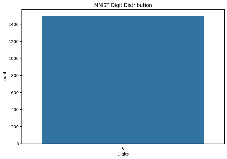
还要检查训练数据中数字的分布,以验证每个类均在数据集中得到合理表示。
sns.countplot(y_viz.numpy());
plt.xlabel('Digits')
plt.title("MNIST Digit Distribution");
预处理数据
首先,通过展平图像将特征矩阵重塑为二维。接下来,重新缩放数据,使 [0,255] 区间内的像素值拟合至 [0,1] 区间内。此步骤可确保输入像素具有相似的分布并有助于训练收敛。
def preprocess(x, y):
  # Reshaping the data
  x = tf.reshape(x, shape=[-1, 784])
  # Rescaling the data
  x = x/255
  return x, y

train_data, val_data = train_data.map(preprocess), val_data.map(preprocess)
构建 MLP
首先,呈现 ReLU 和 Softmax 激活函数。这两个函数分别在 tf.nn.relu 和 tf.nn.softmax 中提供。ReLU 是一个非线性激活函数,会在输入值为正的情况下输出输入值,否则输出 0:
\[\text{ReLU}(X) = max(0, X)\]
x = tf.linspace(-2, 2, 201)
x = tf.cast(x, tf.float32)
plt.plot(x, tf.nn.relu(x));
plt.xlabel('x')
plt.ylabel('ReLU(x)')
plt.title('ReLU activation function');

softmax 激活函数是一个归一化指数函数,可以将 \(m\) 个实数转换为具有 \(m\) 个结果/类的概率分布。这在从神经网络的输出预测类概率方面非常实用:
\[\text{Softmax}(X) = \frac{e^{X} }{\sum_{i=1}^{m}e^{X_i} }\]
x = tf.linspace(-4, 4, 201)
x = tf.cast(x, tf.float32)
plt.plot(x, tf.nn.softmax(x, axis=0));
plt.xlabel('x')
plt.ylabel('Softmax(x)')
plt.title('Softmax activation function');

密集层
为密集层创建一个类。根据定义,在 MLP 中,一层的输出将完全连接到下一层的输入。因此,密集层的输入维度可以根据其前一层的输出维度进行推断,并且不需要在其初始化期间预先指定。权重也应正确初始化,以防止激活输出变得过大或过小。最热门的权重初始化方法之一是 Xavier 方案,其中权重矩阵的每个元素都以下列方式进行采样:
\[W_{ij} \sim \text{Uniform}(-\frac{\sqrt{6} }{\sqrt{n + m} },\frac{\sqrt{6} }{\sqrt{n + m} })\]
偏差向量可初始化为零。
def xavier_init(shape):
  # Computes the xavier initialization values for a weight matrix
  in_dim, out_dim = shape
  xavier_lim = tf.sqrt(6.)/tf.sqrt(tf.cast(in_dim + out_dim, tf.float32))
  weight_vals = tf.random.uniform(shape=(in_dim, out_dim),
                                  minval=-xavier_lim, maxval=xavier_lim, seed=22)
  return weight_vals
Xavier 初始化方法也可以采用 tf.keras.initializers.GlorotUniform 实现。
class DenseLayer(tf.Module):

  def __init__(self, out_dim, weight_init=xavier_init, activation=tf.identity):
    # Initialize the dimensions and activation functions
    self.out_dim = out_dim
    self.weight_init = weight_init
    self.activation = activation
    self.built = False

  def __call__(self, x):
    if not self.built:
      # Infer the input dimension based on first call
      self.in_dim = x.shape[1]
      # Initialize the weights and biases using Xavier scheme
      self.w = tf.Variable(xavier_init(shape=(self.in_dim, self.out_dim)))
      self.b = tf.Variable(tf.zeros(shape=(self.out_dim,)))
      self.built = True
    # Compute the forward pass
    z = tf.add(tf.matmul(x, self.w), self.b)
    return self.activation(z)
接下来,为按顺序执行层的 MLP 模型构建一个类。请谨记,由于维度推断,模型变量只有在第一个密集层调用序列之后才可用。
class MLP(tf.Module):

  def __init__(self, layers):
    self.layers = layers

  @tf.function
  def __call__(self, x, preds=False):
    # Execute the model's layers sequentially
    for layer in self.layers:
      x = layer(x)
    return x
初始化具有以下架构的 MLP 模型:
- 前向传递:ReLU(784 x 700) x ReLU(700 x 500) x Softmax(500 x 10)
softmax 激活函数不需要由 MLP 应用。它会在损失函数和预测函数中分别计算。
hidden_layer_1_size = 700
hidden_layer_2_size = 500
output_size = 10

mlp_model = MLP([
    DenseLayer(out_dim=hidden_layer_1_size, activation=tf.nn.relu),
    DenseLayer(out_dim=hidden_layer_2_size, activation=tf.nn.relu),
    DenseLayer(out_dim=output_size)])
定义损失函数
交叉熵损失函数是处理多类分类问题的绝佳选择,因为它会根据模型的概率预测来衡量数据的负对数似然。分配给真实类的概率越高,损失则越低。交叉熵损失的方程如下:
\[L = -\frac{1}{n}\sum_{i=1}^{n}\sum_{i=j}^{n} {y_j}^{[i]}⋅\log(\hat{ {y_j} }^{[i]})\]
其中
- \(\underset{n\times m}{\hat{y} }\):预测类分布的矩阵
- \(\underset{n\times m}{y}\):真实类的独热编码矩阵
tf.nn.sparse_softmax_cross_entropy_with_logits 函数可用于计算交叉熵损失。此函数不需要模型的最后一层应用 softmax 激活函数,也不需要对类标签进行独热编码
def cross_entropy_loss(y_pred, y):
  # Compute cross entropy loss with a sparse operation
  sparse_ce = tf.nn.sparse_softmax_cross_entropy_with_logits(labels=y, logits=y_pred)
  return tf.reduce_mean(sparse_ce)
编写一个基本的准确率函数,计算训练期间正确分类的比例。为了从 softmax 输出生成类预测,返回与最大类概率相对应的索引。
def accuracy(y_pred, y):
  # Compute accuracy after extracting class predictions
  class_preds = tf.argmax(tf.nn.softmax(y_pred), axis=1)
  is_equal = tf.equal(y, class_preds)
  return tf.reduce_mean(tf.cast(is_equal, tf.float32))
训练模型
与标准梯度下降相比,使用优化器可以显著加快收敛速度。Adam 优化器实现方式如下。请参阅优化器指南,以详细了解如何使用 TensorFlow Core 设计自定义优化器。
class Adam:

    def __init__(self, learning_rate=1e-3, beta_1=0.9, beta_2=0.999, ep=1e-7):
      # Initialize optimizer parameters and variable slots
      self.beta_1 = beta_1
      self.beta_2 = beta_2
      self.learning_rate = learning_rate
      self.ep = ep
      self.t = 1.
      self.v_dvar, self.s_dvar = [], []
      self.built = False

    def apply_gradients(self, grads, vars):
      # Initialize variables on the first call
      if not self.built:
        for var in vars:
          v = tf.Variable(tf.zeros(shape=var.shape))
          s = tf.Variable(tf.zeros(shape=var.shape))
          self.v_dvar.append(v